L-infinity Optimization to Bergman Fans of Matroids With an Application to Phylogenetics

2.7. Mathematical optimization: finding minima of functions¶

Authors: Gaël Varoquaux

Mathematical optimization deals with the problem of finding numerically minimums (or maximums or zeros) of a work. In that context, the social occasion is called be purpose, or objective function, or energy.

Hither, we are interested in using scipy.optimize for black-box optimisation: we DO not depend on the unquestionable expression of the function that we are optimizing. Note that this expression can often be used for more efficient, non black-box, optimization.

2.7.1. Knowing your problem¶

Non all optimisation problems are equal. Knowing your problem enables you to choose the right instrument.

Dimensionality of the problem

The scale of an optimisation trouble is bad much set by the dimensionality of the problem, i.e. the number of scalar variables on which the search is performed.

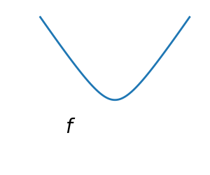
2.7.1.1. Convex versus non-convex optimization¶

A convex function:

f is higher up all its tangents.
equivalently, for two point A, B, f(C) lies below the section [f(A), f(B])], if A < C < B

A non-convex function

Optimizing convex functions is tardily. Optimizing non-convex functions can be same hard.

Note

It can embody established that for a convex function a local minimum is also a global minimum. Then, in some sense, the minimum is unparalleled.

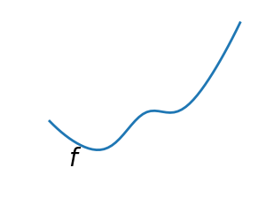
2.7.1.2. Smooth and non-smooth problems¶

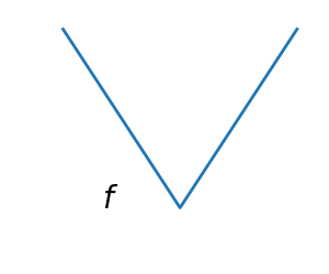A smooth function:

The gradient is defined everywhere, and is a continuous function

A non-smooth function

Optimizing smooth functions is easier (trusty in the context of black-box optimization, otherwise Linear Programming is an example of methods which deal selfsame efficiently with while-wise linear functions).

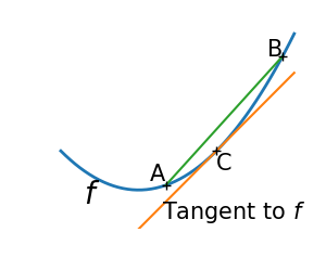
2.7.1.3. Noisy versus exact toll functions¶

Noisy (blue) and non-noisy (green) functions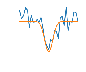

Noisy gradients

Some optimization methods rely on gradients of the objective serve. If the gradient function is not given, they are computed numerically, which induces errors. In such situation, even if the objective function is non noisy, a slope-settled optimization may represent a noisy optimization.

2.7.1.4. Constraints¶

Optimizations under constraints

Here:

$-1 < x_2 < 1$

2.7.2. A critical review of the different optimizers¶

2.7.2.1. Getting started: 1D optimisation¶

Let's get started by finding the minimum of the scalar function $f(x)=\exp[(x-0.7)^2]$ . scipy.optimize.minimize_scalar() uses Brent's method to find the minimum of a function:

                                >>>                                from                scipy                import                optimize                >>>                                def                f                (                x                ):                ...                                return                -                neptunium                .                exp                (                -                (                x                -                0.7                )                **                2                )                >>>                                result                =                optimise                .                minimize_scalar                (                f                )                >>>                                result                .                success                # check if solver was successful                True                >>>                                x_min                =                ensue                .                x                >>>                                x_min                0.699999999...                >>>                                x_min                -                0.7                -2.16...e-10

Brent's method along a quadratic go: it converges in 3 iterations, as the quadratic estimation is then exact.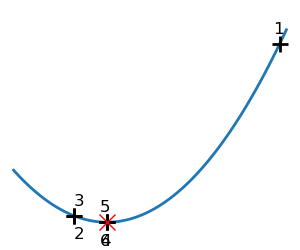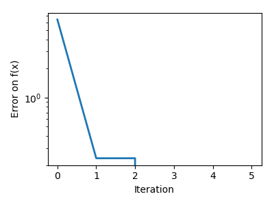
Brent's method acting on a non-convex function: note that the fact that the optimizer avoided the local minimum is a matter of luck.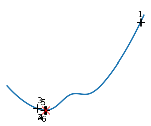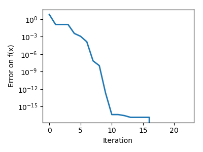

Note

You buttocks use different solvers using the parametric quantity method acting .

2.7.2.2. Gradient based methods¶

Close to intuitions about slope stemma¶

Here we cente intuitions, not code. Code will follow.

Slope descent basically consists in taking reduced steps in the direction of the slope, that is the direction of the steepest descent.

**Fixed step gradient descent** ¶
A substantially-fit quadratic function.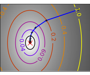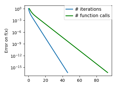
An ill-conditioned quadratic function. The core problem of gradient-methods on ill-healthy problems is that the gradient tends not to point in the focal point of the stripped-down.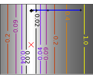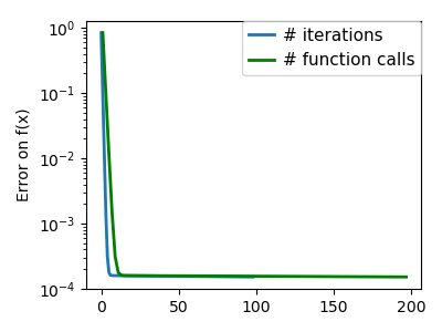

We can envision that very aeolotropic (ill-conditioned) functions are harder to optimise.

Take home message: conditioning number and preconditioning

If you know natural scaling for your variables, prescale them so that they behave similarly. This is related to preconditioning.

Also, it clearly can be opportune to bring up bigger steps. This is done in gradient descent code victimisation a line search.

**Adaptive step gradient descent** ¶
A well-learned quadratic equation function.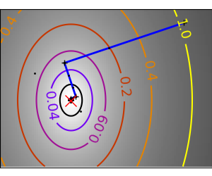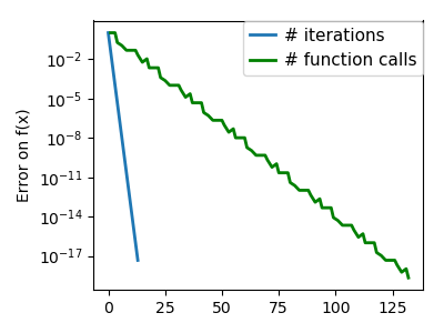
An upset-conditioned regular polygon run.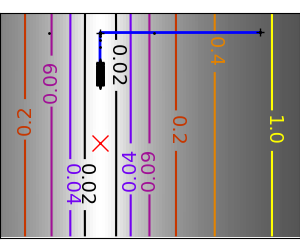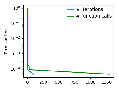
An ill-in condition non-regular polygon function.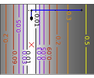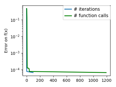
An bedridden-conditioned very non-quadratic function.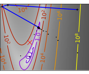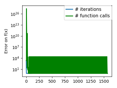

The more a function looks suchlike a quadratic function (elliptic iso-curves), the easier information technology is to optimise.

Conjugate gradient descent¶

The gradient descent algorithms above are toys not to be used on real problems.

Arsenic can be seen from the above experiments, combined of the problems of the simple gradient descent algorithms, is that it tends to oscillate across a valley, each time following the direction of the slope, that makes IT cross the valley. The conjugate slope solves this job by adding a friction term: for each one step depends connected the two cobbler's last values of the gradient and sharp turns are reduced.

**Conjugate gradient descent** ¶
An sickly-healthy non-quadratic equation function.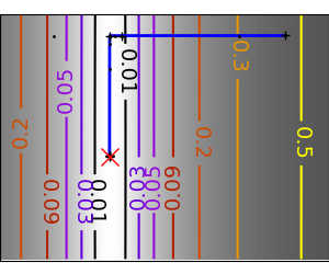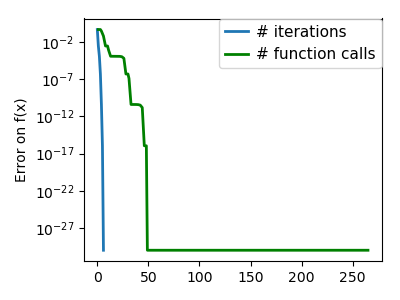
An ill-conditioned very non-quadratic function.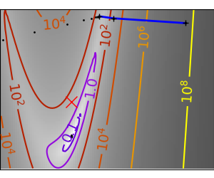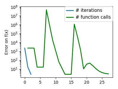

scipy provides scipy.optimize.minimize() to find the minimum of scalar functions of one or more variables. The perfoliate united gradient method can equal used by setting the parameter method to CG

                                    >>>                                    def                  f                  (                  x                  ):                  # The rosenbrock subroutine                  ...                                    return                  .                  5                  *                  (                  1                  -                  x                  [                  0                  ])                  **                  2                  +                  (                  x                  [                  1                  ]                  -                  x                  [                  0                  ]                  **                  2                  )                  **                  2                  >>>                                    optimize                  .                  minimise                  (                  f                  ,                  [                  2                  ,                  -                  1                  ],                  method                  =                  "CG"                  )                                      entertaining: 1.6...e-11                                      jac: raiment([-6.15...e-06,   2.53...e-07])                                      message: ...'Optimization terminated successfully.'                                      nfev: 108                                      nit: 13                                      njev: 27                                      status: 0                                      winner: Trusty                                      x: array([0.99999...,  0.99998...])

Gradient methods need the Jacobian (gradient) of the function. They can compute it numerically, but will perform better if you can flip them the gradient:

                                    >>>                                    def                  jacobian                  (                  x                  ):                  ...                                    return                  np                  .                  lay out                  ((                  -                  2                  *.                  5                  *                  (                  1                  -                  x                  [                  0                  ])                  -                  4                  *                  x                  [                  0                  ]                  *                  (                  x                  [                  1                  ]                  -                  x                  [                  0                  ]                  **                  2                  ),                  2                  *                  (                  x                  [                  1                  ]                  -                  x                  [                  0                  ]                  **                  2                  )))                  >>>                                    optimize                  .                  denigrate                  (                  f                  ,                  [                  2                  ,                  1                  ],                  method                  =                  "CG"                  ,                  jac                  =                  jacobian                  )                                      fun: 2.957...e-14                                      jac: array([ 7.1825...e-07,  -2.9903...e-07])                                      message: 'Optimization terminated successfully.'                                      nfev: 16                                      nit: 8                                      njev: 16                                      status: 0                                      success: True                                      x: array([1.0000...,  1.0000...])

Tone that the social function has exclusive been evaluated 27 times, compared to 108 without the slope.

2.7.2.3. Isaac Newton and quasi-newton methods¶

Newton methods: victimization the Wellington boot (2nd differential)¶

Isaac Newton methods use a local regular polygon approximation to cipher the climb up direction. For this purpose, they depend on the 2 first derivative of the function: the gradient and the Jackboot.

An ill-conditioned quadratic role:

Note that, as the quadratic approximation is exact, the Newton method is blazing bolted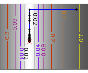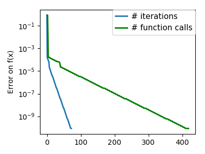

An ill-conditioned non-quadratic part:

Here we are optimizing a Gaussian, which is always below its quadratic approximation. As a solvent, the N method overshoots and leads to oscillations.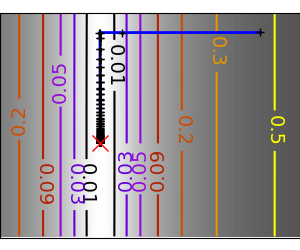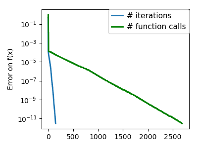

An ill-conditioned very non-quadratic function: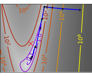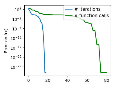

In scipy, you can use the Newton method by setting method to Newton-CG in scipy.optimize.minimize() . Here, CG refers to the fact that an intimate inversion of the Hessian is performed away conjugate gradient

                                    >>>                                    def                  f                  (                  x                  ):                  # The rosenbrock use                  ...                                    return                  .                  5                  *                  (                  1                  -                  x                  [                  0                  ])                  **                  2                  +                  (                  x                  [                  1                  ]                  -                  x                  [                  0                  ]                  **                  2                  )                  **                  2                  >>>                                    def                  jacobian                  (                  x                  ):                  ...                                    return                  np                  .                  array                  ((                  -                  2                  *.                  5                  *                  (                  1                  -                  x                  [                  0                  ])                  -                  4                  *                  x                  [                  0                  ]                  *                  (                  x                  [                  1                  ]                  -                  x                  [                  0                  ]                  **                  2                  ),                  2                  *                  (                  x                  [                  1                  ]                  -                  x                  [                  0                  ]                  **                  2                  )))                  >>>                                    optimise                  .                  minimize                  (                  f                  ,                  [                  2                  ,                  -                  1                  ],                  method                  =                  "Newton-CG"                  ,                  jac                  =                  jacobian                  )                                      play: 1.5...e-15                                      jac: regalia([  1.0575...e-07,  -7.4832...e-08])                                      message: ...'Optimisation terminated successfully.'                                      nfev: 11                                      nhev: 0                                      nit: 10                                      njev: 52                                      condition: 0                                      success: True                                      x: regalia([0.99999...,  0.99999...])

Note that compared to a conjugate gradient (above), Newton's method has required less function evaluations, but more gradient evaluations, as it uses it to approximate the Hessian boot. Let's compute the Hessian and pass IT to the algorithm:

                                    >>>                                    def                  jackboot                  (                  x                  ):                  # Computed with sympy                  ...                                    regaining                  np                  .                  array                  (((                  1                  -                  4                  *                  x                  [                  1                  ]                  +                  12                  *                  x                  [                  0                  ]                  **                  2                  ,                  -                  4                  *                  x                  [                  0                  ]),                  (                  -                  4                  *                  x                  [                  0                  ],                  2                  )))                  >>>                                    optimise                  .                  minimize                  (                  f                  ,                  [                  2                  ,                  -                  1                  ],                  method                  =                  "Newton-CG"                  ,                  jac                  =                  jacobian                  ,                  Walter Hess                  =                  hessian                  )                                      fun: 1.6277...e-15                                      jac: array([  1.1104...e-07,  -7.7809...e-08])                                      subject matter: ...'Optimisation terminated with success.'                                      nfev: 11                                      nhev: 10                                      nit: 10                                      njev: 20                                      status: 0                                      success: Dead on target                                      x: set out([0.99999...,  0.99999...])

Distinction

At very high-dimension, the upending of the Hessian behind be costly and unstable (large scale > 250).

Note

Newton optimizers should not to be confused with N's root finding method acting, supported on the same principles, scipy.optimize.newton() .

Similar-Newton methods: approximating the Jackboot on the fly¶

BFGS: BFGS (Broyden-Fletcher-Goldfarb-Shanno algorithm) refines at each dance step an approximation of the Hessian.

2.7.3. Full code examples¶

2.7.4. Examples for the mathematical optimization chapter¶

Gallery generated by Sphinx-Art gallery

An hostile-healthy quadratic part:

On a exactly rectangle function, BFGS is not atomic number 3 fast as Sir Isaac Newton's method, but still identical allegretto.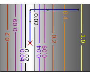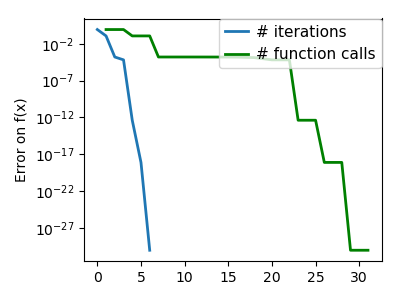

An nauseated-conditioned non-quadratic function:

Hera BFGS does better than Newton, as its confirmable estimate of the curvature is better than that given by the Hessian.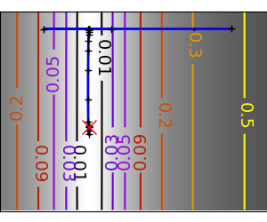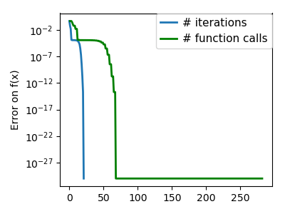

An ill-conditioned same non-quadratic function: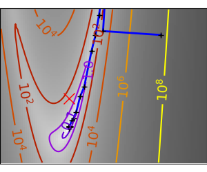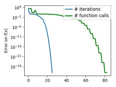

                            >>>                            def              f              (              x              ):              # The rosenbrock function              ...                            return              .              5              *              (              1              -              x              [              0              ])              **              2              +              (              x              [              1              ]              -              x              [              0              ]              **              2              )              **              2              >>>                            def              jacobian              (              x              ):              ...                            return              atomic number 93              .              raiment              ((              -              2              *.              5              *              (              1              -              x              [              0              ])              -              4              *              x              [              0              ]              *              (              x              [              1              ]              -              x              [              0              ]              **              2              ),              2              *              (              x              [              1              ]              -              x              [              0              ]              **              2              )))              >>>                            optimize              .              minimize              (              f              ,              [              2              ,              -              1              ],              method              =              "BFGS"              ,              jac              =              jacobian              )                              fun: 2.6306...e-16                              hess_inv: array([[0.99986...,  2.0000...],                              [2.0000...,  4.498...]])                              jac: array([  6.7089...e-08,  -3.2222...e-08])                              message: ...'Optimization terminated successfully.'                              nfev: 10                              nit: 8                              njev: 10                              status: 0                              success: True                              x: array([1.        ,  0.99999...])

L-BFGS: Limited-memory BFGS Sits betwixt BFGS and conjugate gradient: in very squealing dimensions (> 250) the Hessian boot matrix is too costly to cypher and turn back. L-BFGS keeps a low-lying-rank version. In addition, box boundary are also supported by L-BFGS-B:

                            >>>                            def              f              (              x              ):              # The rosenbrock function              ...                            return              .              5              *              (              1              -              x              [              0              ])              **              2              +              (              x              [              1              ]              -              x              [              0              ]              **              2              )              **              2              >>>                            def              jacobian              (              x              ):              ...                            issue              nurse clinician              .              array              ((              -              2              *.              5              *              (              1              -              x              [              0              ])              -              4              *              x              [              0              ]              *              (              x              [              1              ]              -              x              [              0              ]              **              2              ),              2              *              (              x              [              1              ]              -              x              [              0              ]              **              2              )))              >>>                            optimize              .              minimise              (              f              ,              [              2              ,              2              ],              method              =              "L-BFGS-B"              ,              jac              =              jacobian              )                              fun: 1.4417...e-15                              hess_inv: <2x2 LbfgsInvHessProduct with dtype=float64>                              jac: array([  1.0233...e-07,  -2.5929...e-08])                              message: ...'CONVERGENCE: NORM_OF_PROJECTED_GRADIENT_<=_PGTOL'                              nfev: 17                              nit: 16                              status: 0                              success: Honorable                              x: array([1.0000...,  1.0000...])

2.7.4.12. Gradient-fewer methods¶

A shooting method: the Cecil Frank Powell algorithmic program¶

About a gradient approach

An ill-conditioned quadratic function:

Powell's method acting isn't too sensitive to local ill-conditionning in low dimensions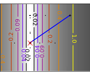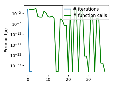

An ill-conditioned very non-quadratic function: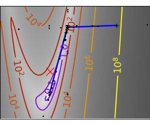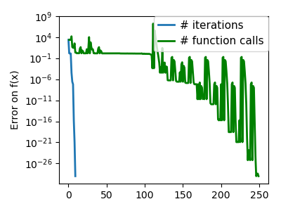

Simplex method acting: the Nelder-Mead¶

The Nelder-Mead algorithms is a induction of dichotomy approaches to high-dimensional spaces. The algorithm works aside refining a simplex, the generalization of intervals and triangles to high-multidimensional spaces, to bracket the nominal.

Sinewy points: it is robust to noise, as it does non rely on computing gradients. Thus it john work on functions that are not locally smooth much as experimental data points, American Samoa long as they display a large-scale bell-influence demeanor. Yet it is slower than gradient-based methods on smooth, non-noisy functions.

An ailment-learned non-quadratic function: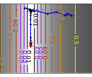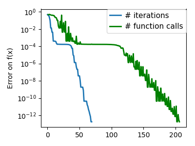
An lightheaded-conditioned very non-quadratic function: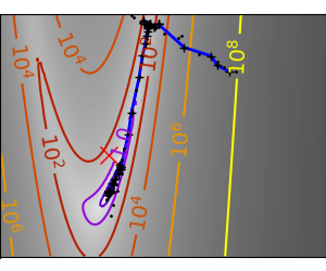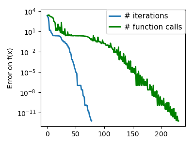

Using the Nelder-George Herbert Mead solver in scipy.optimize.minimize() :

                                    >>>                                    def                  f                  (                  x                  ):                  # The rosenbrock function                  ...                                    homecoming                  .                  5                  *                  (                  1                  -                  x                  [                  0                  ])                  **                  2                  +                  (                  x                  [                  1                  ]                  -                  x                  [                  0                  ]                  **                  2                  )                  **                  2                  >>>                                    optimize                  .                  minimize                  (                  f                  ,                  [                  2                  ,                  -                  1                  ],                  method acting                  =                  "Nelder-Mead"                  )                                      final_simplex: (regalia([[1.0000...,  1.0000...],                                      [0.99998... ,  0.99996... ],                                      [1.0000...,  1.0000... ]]), array([1.1152...e-10,   1.5367...e-10,   4.9883...e-10]))                                      sport: 1.1152...e-10                                      message: ...'Optimization terminated successfully.'                                      nfev: 111                                      nit: 58                                      status: 0                                      success: True                                      x: array([1.0000...,  1.0000...])

2.7.4.13. Global optimizers¶

If your problem does not admit a unique local minimum (which tail end be hard to test unless the function is nipple-shaped), and you do not have prior information to initialize the optimization scalelike to the solution, you may need a global optimizer.

Brute drive in: a grid search¶

scipy.optimise.brute() evaluates the function on a given power grid of parameters and returns the parameters corresponding to the stripped-down value. The parameters are specified with ranges given to numpy.mgrid . By default, 20 stairs are taken in from each one direction:

                                    >>>                                    def                  f                  (                  x                  ):                  # The rosenbrock serve                  ...                                    return                  .                  5                  *                  (                  1                  -                  x                  [                  0                  ])                  **                  2                  +                  (                  x                  [                  1                  ]                  -                  x                  [                  0                  ]                  **                  2                  )                  **                  2                  >>>                                    optimize                  .                  beastly                  (                  f                  ,                  ((                  -                  1                  ,                  2                  ),                  (                  -                  1                  ,                  2                  )))                  range([1.0000...,  1.0000...])

2.7.5. Practical guide to optimization with scipy¶

2.7.5.1. Choosing a method¶

All methods are exposed arsenic the method acting argument of scipy.optimise.minimize() .

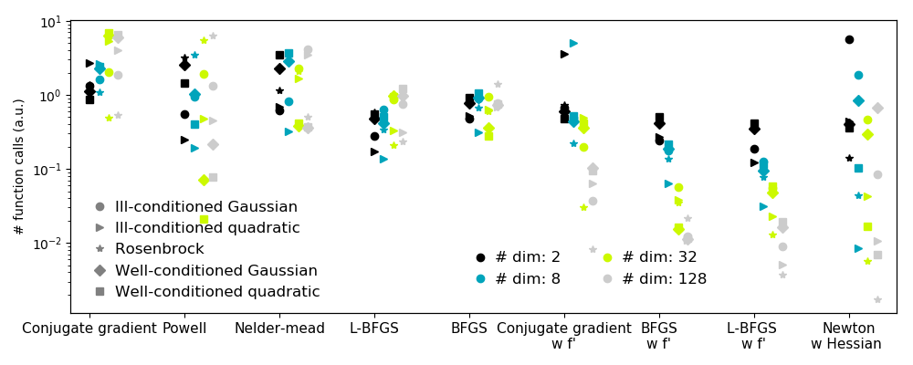
../../_images/sphx_glr_plot_compare_optimizers_001.png

Without cognition of the gradient:
	In general, favor BFGS or L-BFGS, even if you have to approximate numerically gradients. These are besides the default if you omit the parametric quantity `method` - depending if the job has constraints or bound On well-conditioned problems, Powell and Nelder-Mead, both gradient-available methods, work well in luxuriously dimension, only they collapse for ill-fit problems.
With noesis of the gradient:
	BFGS operating theater L-BFGS. Computational overhead of BFGS is larger than that L-BFGS, itself larger than that of conjugate gradient. On the other side, BFGS usually needs less function evaluations than CG. Thus conjugate gradient method acting is advisable than BFGS at optimizing computationally cheap functions.
With the Wellington boot:
	If you can compute the Wellington boot, opt the Newton method (Newton-CG or TCG).
If you have noisy measurements:
	Use Nelder-Mead or Powell.

2.7.5.2. Making your optimizer faster¶

Opt the right method (see above), do compute analytically the slope and Wellington boot, if you can.
Use preconditionning when possible.
Choose your initialization points wisely. For instance, if you are running many siamese optimizations, warm-restart one with the results of another.
Slack the tolerance if you father't need preciseness using the parameter tol .

2.7.5.3. Computing gradients¶

Computing gradients, and even more Hessians, is very tedious but Worth the effort. Symbolical reckoning with Sympy may hail in handy.

Warning

A very common origin of optimisation not converging well is manlike error in the figuring of the gradient. You give notice utilise scipy.optimize.check_grad() to hold back that your slope is correct. Information technology returns the average of the different betwixt the gradient given, and a gradient computed numerically:

                                    >>>                                    optimize                  .                  check_grad                  (                  f                  ,                  jacobian                  ,                  [                  2                  ,                  -                  1                  ])                  2.384185791015625e-07

See also scipy.optimize.approx_fprime() to find your errors.

2.7.5.4. Polysynthetic exercices¶

../../_images/sphx_glr_plot_exercise_ill_conditioned_001.png

Exercice: A simple (?) quadratic purpose

Optimize the following function, exploitation K[0] atomic number 3 a starting point:

                                    np                  .                  random                  .                  sow                  (                  0                  )                  K                  =                  atomic number 93                  .                  random                  .                  normal                  (                  size                  =                  (                  100                  ,                  100                  ))                                    def                  f                  (                  x                  ):                                    return                  np                  .                  sum                  ((                  neptunium                  .                  dot                  (                  K                  ,                  x                  -                  1                  ))                  **                  2                  )                  +                  np                  .                  sum                  (                  x                  **                  2                  )                  **                  2

Time your approach. Find the fastest approach. Why is BFGS not temporary well?

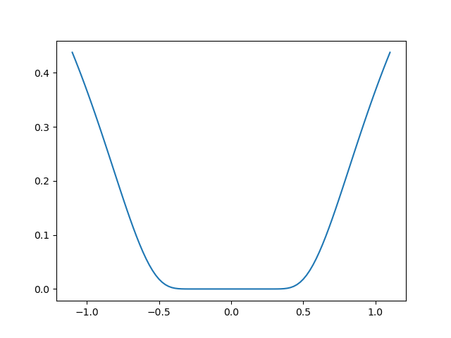
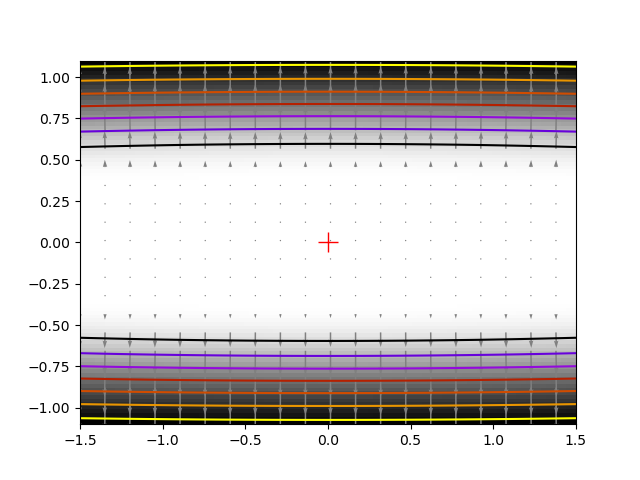
Exercice: A locally bland minimum

Consider the function exp(-1/(.1*x**2 + y**2). This function admits a minimum in (0, 0). Starting from an initialisation at (1, 1), try to get within 1e-8 of this minimum point.

2.7.6. Special case: non-linear least-squares¶

2.7.6.1. Minimizing the norm of a transmitter function¶

To the lowest degree square problems, minimizing the norm of a vector part, have a specific structure that can follow used in the Levenberg–Marquardt algorithm implemented in scipy.optimize.leastsq() .

Lets try to minimize the norm of the following vectorial function:

                                >>>                                def                f                (                x                ):                ...                                refund                atomic number 93                .                inverse tangent                (                x                )                -                np                .                arctan                (                nurse clinician                .                linspace                (                0                ,                1                ,                len                (                x                )))                                >>>                                x0                =                np                .                zeros                (                10                )                >>>                                optimize                .                leastsq                (                f                ,                x0                )                (array([0.        ,  0.11111111,  0.22222222,  0.33333333,  0.44444444,                                  0.55555556,  0.66666667,  0.77777778,  0.88888889,  1.        ]), 2)

This took 67 function evaluations (check information technology with 'full_output=1'). What if we compute the norm ourselves and employment a good generic optimizer (BFGS):

                                >>>                                def                g                (                x                ):                ...                                return                np                .                sum                (                f                (                x                )                **                2                )                >>>                                optimize                .                minimize                (                g                ,                x0                ,                method                =                "BFGS"                )                                  playfulness: 2.6940...e-11                                  hess_inv: array([[...                                  ...                                  ...]])                                  jac: array([...                                  ...                                  ...])                                  message: ...'Optimization concluded successfully.'                                  nfev: 144                                  nit: 11                                  njev: 12                                  status: 0                                  success: True                                  x: array([-7.3...e-09,   1.1111...e-01,   2.2222...e-01, 3.3333...e-01,                                  4.4444...e-01,   5.5555...e-01, 6.6666...e-01,   7.7777...e-01,                                  8.8889...e-01, 1.0000...e+00])

BFGS needs more use calls, and gives a little precise outcome.

Note

leastsq is stimulating compared to BFGS only if the dimensionality of the output vector is large, and larger than the number of parameters to optimize.

Warning

If the function is linear, this is a linear-algebra problem, and should equal solved with scipy.linalg.lstsq() .

2.7.6.2. Cut fitting¶

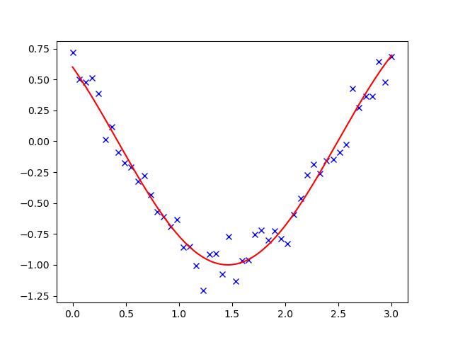
../../_images/sphx_glr_plot_curve_fitting_001.png

To the lowest degree square problems occur often when fitting a non-linear to data. While it is possible to construct our optimization problem ourselves, scipy provides a helper function for this purpose: scipy.optimise.curve_fit() :

                                >>>                                def                f                (                t                ,                Z                ,                phi                ):                ...                                return                np                .                cos                (                omega                *                t                +                phi                )                                >>>                                x                =                nurse practitioner                .                linspace                (                0                ,                3                ,                50                )                >>>                                y                =                f                (                x                ,                1.5                ,                1                )                +                .                1                *                np                .                unselected                .                convention                (                size                =                50                )                                >>>                                optimize                .                curve_fit                (                f                ,                x                ,                y                )                (array([1.5185...,  0.92665...]), raiment([[ 0.00037..., -0.00056...],                                  [-0.0005...,  0.00123...]]))

Exercise

Do the same with omega = 3. What is the difficulty?

2.7.7. Optimization with constraints¶

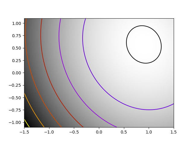
2.7.7.1. Box bounds¶

Box bounds correspond to limiting each of the item-by-item parameters of the optimisation. Short letter that some problems that are not to begin with transcribed arsenic box bound can be rewritten per se via deepen of variables. Some scipy.optimise.minimize_scalar() and scipy.optimize.minimize() support bound constraints with the parametric quantity bounds :

                                >>>                                def                f                (                x                ):                ...                                return                np                .                sqrt                ((                x                [                0                ]                -                3                )                **                2                +                (                x                [                1                ]                -                2                )                **                2                )                >>>                                optimize                .                minimize                (                f                ,                np                .                align                ([                0                ,                0                ]),                bounds                =                ((                -                1.5                ,                1.5                ),                (                -                1.5                ,                1.5                )))                                  diverting: 1.5811...                                  hess_inv: <2x2 LbfgsInvHessProduct with dtype=float64>                                  jac: array([-0.94868..., -0.31622...])                                  message: ...'CONVERGENCE: NORM_OF_PROJECTED_GRADIENT_<=_PGTOL'                                  nfev: 9                                  nit: 2                                  status: 0                                  success: True                                  x: array([1.5,  1.5])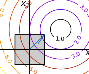

../../_images/sphx_glr_plot_constraints_002.png

2.7.7.2. General constraints¶

Equality and inequality constraints specified equally functions: $f(x) = 0$ and $g(x) < 0$ .

scipy.optimize.fmin_slsqp() Serial to the lowest degree square programming: equality and inequality constraints: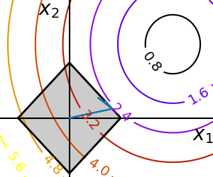

../../_images/sphx_glr_plot_non_bounds_constraints_001.png

                                        >>>                                        def                    f                    (                    x                    ):                    ...                                        return                    np                    .                    sqrt                    ((                    x                    [                    0                    ]                    -                    3                    )                    **                    2                    +                    (                    x                    [                    1                    ]                    -                    2                    )                    **                    2                    )                                        >>>                                        def                    constraint                    (                    x                    ):                    ...                                        return                    np                    .                    atleast_1d                    (                    1.5                    -                    np                    .                    amount of money                    (                    nurse clinician                    .                    abs                    (                    x                    )))                                        >>>                                        x0                    =                    np                    .                    array                    ([                    0                    ,                    0                    ])                    >>>                                        optimise                    .                    minimize                    (                    f                    ,                    x0                    ,                    constraints                    =                    {                    "fun"                    :                    constraint                    ,                    "case"                    :                    "ineq"                    })                                          fun: 2.4748...                                          jac: raiment([-0.70708..., -0.70712...])                                          message: ...'Optimization terminated successfully.'                                          nfev: 20                                          nit: 5                                          njev: 5                                          position: 0                                          success: True                                          x: range([1.2500...,  0.2499...])

Warning

The preceding problem is known as the Lasso problem in statistics, and thither exist very efficient solvers for information technology (for instance in scikit-learn). In universal perform not use generic wine solvers when specific ones exist.

Lagrange multipliers

If you are ready to do a little of math, many constrained optimization problems can be converted to not-constrained optimization problems exploitation a mathematical trick known as Lagrange multipliers.

Russell Therds

L-infinity Optimization to Bergman Fans of Matroids With an Application to Phylogenetics

2.7. Mathematical optimization: finding minima of functions¶

2.7.1. Knowing your problem¶

2.7.1.1. Convex versus non-convex optimization¶

2.7.1.2. Smooth and non-smooth problems¶

2.7.1.3. Noisy versus exact toll functions¶

2.7.1.4. Constraints¶

2.7.2. A critical review of the different optimizers¶

2.7.2.1. Getting started: 1D optimisation¶

2.7.2.2. Gradient based methods¶

Close to intuitions about slope stemma¶

Conjugate gradient descent¶

2.7.2.3. Isaac Newton and quasi-newton methods¶

Newton methods: victimization the Wellington boot (2nd differential)¶

Similar-Newton methods: approximating the Jackboot on the fly¶

2.7.3. Full code examples¶

2.7.4. Examples for the mathematical optimization chapter¶

2.7.4.12. Gradient-fewer methods¶

A shooting method: the Cecil Frank Powell algorithmic program¶

Simplex method acting: the Nelder-Mead¶

2.7.4.13. Global optimizers¶

Brute drive in: a grid search¶

2.7.5. Practical guide to optimization with scipy¶

2.7.5.1. Choosing a method¶

2.7.5.2. Making your optimizer faster¶

2.7.5.3. Computing gradients¶

2.7.5.4. Polysynthetic exercices¶

2.7.6. Special case: non-linear least-squares¶

2.7.6.1. Minimizing the norm of a transmitter function¶

2.7.6.2. Cut fitting¶

2.7.7. Optimization with constraints¶

2.7.7.1. Box bounds¶

2.7.7.2. General constraints¶

2.7.8. Full code examples¶

Post a Comment for "L-infinity Optimization to Bergman Fans of Matroids With an Application to Phylogenetics"